[Home]

Flow Network based Generative Models for Non-Iterative Diverse Candidate Generation

Emmanuel Bengio, Moksh Jain, Maksym Korablyov, Doina Precup, Yoshua Bengio
arXiv preprint, code
also see the GFlowNet Foundations paper
and a more recent (and thorough) tutorial on the framework
and this colab tutorial.
What follows is a high-level overview of this work, for more details refer to our paper. Given a reward $R(x)$ and a deterministic episodic environment where episodes end with a ``generate $x$'' action, how do we generate diverse and high-reward $x$s?
We propose to use Flow Networks to model discrete $p(x) \propto R(x)$ from which we can sample sequentially (like episodic RL, rather than iteratively as MCMC methods would). We show that our method, GFlowNet, is very useful on a combinatorial domain, drug molecule synthesis, because unlike RL methods it generates diverse $x$s by design.

Flow Networks

A flow network is a directed graph with sources and sinks, and edges carrying some amount of flow between them through intermediate nodes -- think of pipes of water. For our purposes, we define a flow network with a single source, the root or $s_0$; the sinks of the network correspond to the terminal states. We'll assign to each sink $x$ an ``out-flow'' $R(x)$.

Given the graph structure and the out-flow of the sinks, we wish to calculate a valid flow between nodes, e.g. how much water each pipe is carrying. Generally there can be infinite solutions, but this is not a problem here -- any valid solution will do. For example above, there is almost no flow between $s_7$ and $s_{13}$ that goes through $s_{11}$, it all goes through $s_{10}$, but the reverse solution would also be a valid flow.
Why is this useful? Such a construction corresponds to a generative model. If we follow the flow, we'll end up in a terminal state, a sink, with probability $p(x) \propto R(x)$. On top of that, we'll have the property that the in-flow of $s_0$--the flow of the unique source--is $\sum_x R(x)=Z$, the partition function. If we assign to each intermediate node a state and to each edge an action, we recover a useful MDP.
Let $F(s,a)=f(s,s')$ be the flow between $s$ and $s'$, where $T(s,a)=s'$, i.e. $s'$ is the (deterministic) state transitioned to from state $s$ and action $a$. Let $$\begin{aligned}\pi(a|s) = \frac{F(s,a)}{\sum_{a'}F(s,a')}\end{aligned}$$ then following policy $\pi$, starting from $s_0$, leads to terminal state $x$ with probability $R(x)$ (see the paper for proofs and more rigorous explanations).

Approximating Flow Networks

As you may suspect, there are only few scenarios in which we can build the above graph explicitly. For drug-like molecules, it would have around $10^{16}$ nodes!
Instead, we resort to function approximation, just like deep RL resorts to it when computing the (action-)value functions of MDPs.
Our goal here is to approximate the flow $F(s,a)$. Earlier we called a valid flow one that correctly routed all the flow from the source to the sinks through the intermediary nodes. Let's be more precise. For some node $s'$, let the in-flow $F(s')$ be the sum of incoming flows: $$\begin{aligned}F(s') = \sum_{s,a:T(s,a)=s'} F(s,a)\end{aligned}$$ Here the set $\{s,a:T(s,a)=s'\}$ is the set of state-action pairs that lead to $s'$. Now, let the out-flow be the sum of outgoing flows--or the reward if $s'$ is terminal: $$\begin{aligned}F(s') = R(s') + \sum_{a'\in\mathcal{A}(s')} F(s',a').\end{aligned}$$ Note that we reused $F(s')$. This is because for a valid flow, the in-flow is equal to the out-flow, i.e. the flow through $s'$, $F(s')$. Here $\mathcal{A}(s)$ is the set of valid actions in state $s$, which is the empty set when $s$ is a sink. $R(s)$ is 0 unless $s$ is a sink, in which case $R(s)>0$.
We can thus call the set of these equalities for all states $s'\neq s_0$ the flow consistency equations: $$\begin{aligned}\sum_{s,a:T(s,a)=s'} F(s,a) = R(s') + \sum_{a'\in\mathcal{A}(s')} F(s',a').\end{aligned}$$

Here the set of parents $\{s,a:T(s,a)=s_3\}$ is $\{(s_0, a_1), (s_1, a_7), (s_2, a_3)\}$, and $\mathcal{A}(s_3)=\{a_2,a_4,a_8\}$.
By now our RL senses should be tingling. We've defined a value function recursively, with two quantities that need to match.

A TD-Like Objective

Just like one can cast the Bellman equations into TD objectives, so do we cast the flow consistency equations into an objective. We want $F_\theta$ that minimizes the square difference between the two sides of the equations, but we add a few bells and whistles: $$\begin{aligned}\mathcal{L}_{\theta,\epsilon}(\tau) = \sum_{\mathclap{s'\in\tau\neq s_0}}\,\left(\log\! \left[\epsilon+{\sum_{\mathclap{s,a:T(s,a)=s'}}} \exp F^{\log}_\theta(s,a)\right]- \log\! \left[\epsilon + R(s') + \sum_{\mathclap{a'\in{\cal A}(s')}} \exp F^{\log}_\theta(s',a')\right]\right)^2.\end{aligned}$$ First, we match the $\log$ of each side, which is important since as intermediate nodes get closer to the root, their flow will become exponentially bigger (remember that $F(s_0) = Z = \sum_x R(x)$), but we care equally about all nodes. Second, we predict $F^{\log}_\theta\approx\log F$ for the same reasons. Finally, we add an $\epsilon$ value inside the $\log$; this doesn't change the minima of the objective, but gives more gradient weight to large values and less to small values.
We show in the paper that a minimizer of this objective achieves our desiderata, which is to have $p(x)\propto R(x)$ when sampling from $\pi(a|s)$ as defined above.

GFlowNet as Amortized Sampling with an OOD Potential

It is interesting to compare GFlowNet with Monte-Carlo Markov Chain (MCMC) methods. MCMC methods can be used to sample from a distribution for which there is no analytical sampling formula but an energy function or unnormalized probability function is available. In our context, this unnormalized probability function is our reward function $R(x)=e^{-energy(x)}$.
Like MCMC methods, GFlowNet can turn a given energy function into samples but it does it in an amortized way, converting the cost a lot of very expensive MCMC trajectories (to obtain each sample) into the cost training a generative model (in our case a generative policy which sequentially builds up $x$). Sampling from the generative model is then very cheap (e.g. adding one component at a time to a molecule) compared to an MCMC. But the most important gain may not be just computational, but in terms of the ability to discover new modes of the reward function.
MCMC methods are iterative, making many small noisy steps, which can converge in the neighborhood of a mode, and with some probability jump from one mode to a nearby one. However, if two modes are far from each other, MCMC can require exponential time to mix between the two. If in addition the modes occupy a tiny volume of the state space, the chances of initializing a chain near one of the unknown modes is also tiny, and the MCMC approach becomes unsatisfactory. Whereas such a situation seems hopeless with MCMC, GFlowNet has the potential to discover modes and jump there directly, if there is structure that relates the modes that it already knows, and if its inductive biases and training procedure make it possible to generalize there.
GFlowNet does not need to perfectly know where the modes are: it is sufficient to make guesses which occasionally work well. Like for MCMC methods, once a point in the region of new mode is discovered, further training of GFlowNet will sculpt that mode and zoom in on its peak.
Note that we can put $R(x)$ to some power $\beta$, a coefficient which acts like a temperature, and $R(x)^\beta = e^{-\beta\; energy(x)}$, making it possible to focus more or less on the highest modes (versus spreading probability mass more uniformly).

Generating molecule graphs

The motivation for this work is to be able to generate diverse molecules from a proxy reward $R$ that is imprecise because it comes from biochemical simulations that have a high uncertainty. As such, we do not care about the maximizer as RL methods would, but rather about a set of ``good enough'' candidates to send to a true biochemical assay.
Another motivation is to have diversity: by fitting the distribution of rewards rather than trying to maximize the expected reward, we're likely to find more modes than if we were being greedy after having found a good enough mode, which again and again we've found RL methods such as PPO to do.
Here we generate molecule graphs via a sequence of additive edits, i.e. we progressively build the graph by adding new leaf nodes to it. We also create molecules block-by-block rather than atom-by-atom.
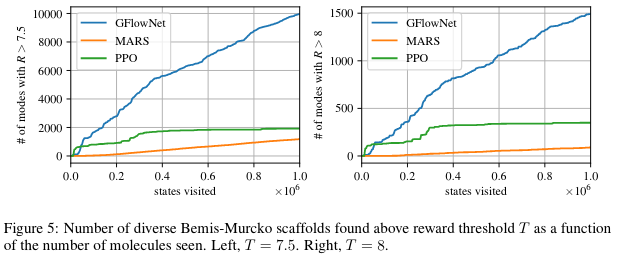
We find experimentally that we get both good molecules, and diverse ones. We compare ourselves to PPO and MARS (an MCMC-based method).
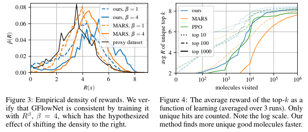
Figure 3 shows that we're fitting a distribution that makes sense. If we change the reward by exponentiating it as $R^\beta$ with $\beta>1$, this shifts the reward distribution to the right.
Figure 4 shows the top-$k$ found as a function of the number of episodes.

Finally, Figure 5 shows that using a biochemical measure of diversity to estimate the number of distinct modes found, GFlowNet finds much more varied candidates.

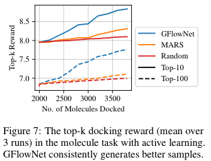
Active Learning experiments

The above experiments assume access to a reward $R$ that is cheap to evaluate. In fact it uses a neural network proxy trained from a large dataset of molecules. This setup isn't quite what we would get when interacting with biochemical assays, where we'd have access to much fewer data. To emulate such a setting, we consider our oracle to be a docking simulation (which is relatively expensive to run, ~30 cpu seconds).
In this setting, there is a limited budget for calls to the true oracle $O$. We use a proxy $M$ initialized by training on a limited dataset of $(x, R(x))$ pairs $D_0$, where $R(x)$ is the true reward from the oracle. The generative model ($\pi_{\theta}$) is then trained to fit $R$ but as predicted by the proxy $M$. We then sample a batch $B=\{x_1, x_2, \dots x_k\}$ where $x_i\sim \pi_{\theta}$, which is evaluated with the oracle $O$. The proxy $M$ is updated with this newly acquired and labeled batch, and the process is repeated for $N$ iterations.
By doing this on the molecule setting we again find that we can generate better molecules. This showcases the importance of having these diverse candidates.

For more figures, experiments and explanations, check out the paper, or reach out to us!