[Home]

Correcting Momentum in Temporal Difference Learning

In this paper we show that momentum becomes stale, especially in TD learning, and we propose a way to correct the staleness. This improves performance on policy evaluation.
See the full paper here.
We consider momentum SGD (Boris T Polyak
Some methods of speeding up the convergence of iteration methods, 1964Boris T Polyak, 1964): We can see momentum as a discounted sum of past gradients, I write here its simplest form for illustration:
What do we mean by ``past gradients''? Let's fold all data (input/target) in $x_t$, and say gradients come from some differentiable function $J$. Then: $$\begin{aligned}g_i = \nabla \theta_i J(\theta_i; x_i)\end{aligned}$$
More generally, consider that we may want to recompute the gradients for some data $x_i$ but for a different set of parameters $\theta_j$, then we write: $$\begin{aligned}g^j_i = \nabla \theta_j J(\theta_j; x_i)\end{aligned}$$
This allows us to imagine some kind of ``ideal'' momentum, which is the discounted sum of the recomputed gradients for the most recent parameters, i.e. the sum of $g^t_i$:
You can think of this as going back in time and recomputing, correcting past gradients:
Here the origin of the gradient arrows are perhaps decieving, since their new (corrected) source really is $\theta_t$ rather than $\theta_i$. This makes the plot a bit more busy though, so I've exaggerated and lerped the gradients for dramatic effect:
The question now becomes, how do you do this without actually recomputing those gradients? If we did, that would cost a lot and in some sense just be equivalent to batch gradient methods.
We know that in DNNs, parameters don't change that quickly, and that, for well-conditioned parameters (which SGD may push DNNs to have, excluding RNNs) gradients don't change very quickly either. As such we should be fine with a local approximation. Taylor expansions are such approximations, and happen to kind of work ok for DNNs (David Balduzzi, Brian McWilliams, Tony Butler-Yeoman
Neural taylor approximations: Convergence and exploration in rectifier networks, 2017David Balduzzi et al., 2017).
So, instead of recomputing $g^t_i$ with our latest parameters $\theta_t$, let's instead consider the Taylor expansion of $g_i$ around $\theta_i$: $$\begin{aligned}g_i(\theta_i + \Delta\theta) \approx g_i + \nabla_{\theta_i} g_i^T \Delta\theta + o(\|\Delta\theta\|^2)\end{aligned}$$
The derivative of $g_i$ turns out to be some kind of Hessian matrix (but not always exactly ``the Hessian'', as we'll see later with TD). We'll call this matrix $Z_i$.
When $\Delta\theta = \theta_t - \theta_i$, then the above term essentially becomes an approximation of $g_i^t$, which we'll call $\hat g_i^t$. $$\begin{aligned}\hat g_i^t = g_i + Z_i^T (\theta_t - \theta_i)\end{aligned}$$
Now we can rewrite our ``ideal'' momentum, but using $\hat g_i^t$ instead of the perfect $g_i^t$, we'll write this as $\hat\mu$: $$\begin{aligned}\hat\mu_t = \sum_i \beta^{t-i} \hat g_i^t\end{aligned}$$
This still looks like we need to recompute the entire sum at each new $t$, but in fact, since $Z_i$ only needs to be computed once, this leads to a recursive algorithm.
$$\begin{aligned} \hat\mu_{t} &= \mu_{t}-\eta_{t}\\ \eta_{t} & = \beta\eta_{t-1}+\alpha\beta \zeta_{t-1}^{\top}\hat\mu_{t-1}\\ \mu_{t} & = g_{t}+\beta{\mu}_{t-1}\\ \zeta_{t} & =Z_{t}+\beta \zeta_{t-1} \end{aligned}$$
You can think of $\eta_t$ as the correction term, the additive term coming from the Taylor expansion. This term is computed by keeping track of a ``momentum'' of the $Z_i$s, which we call $\zeta_t$.
Why is this important for Temporal Difference?
In TD, the objective is something like ($t$ is optimization time, $s,s'$ is the transition): $$\begin{aligned}J_t = (V_\theta(s_t) - (r_t + \gamma \bar V_\theta(s_t')))^2/2 = \delta^2/2\end{aligned}$$
with $\bar V$ meaning we consider it constant when computing gradients. This gives us the following gradient:
$$\begin{aligned}g_t = (V_\theta(s_t) - (r_t + \gamma V_\theta(s_t'))) \nabla_\theta V_\theta(s_t)\end{aligned}$$
Recall that $Z = \nabla_\theta g$. $Z$ roughly measures how $g$ changes as $\theta$ changes. One important thing to notice is that if we update $\theta$, both $V_\theta(s_t)$ and $V_\theta(s_t')$ will change (unless we use frozen targets but we'll assume this is not the case).
This double change means that the gradients accumulated in momentum will be, in a way, doubly stale.
As such, when computing $Z$ we need take take the derivative wrt both $V_\theta(s_t)$ and $V_\theta(s_t')$(meaning $Z\neq \nabla^2 J$). This gives us the following $Z$ for TD: $$\begin{aligned}Z_{TD}=(\nabla_{\theta}V_{\theta}(x)-\gamma\nabla_{\theta}V_{\theta}(x'))\nabla_{\theta}V_{\theta}(x)^T\end{aligned}$$
This allows us not only to correct for ``staleness'', but also corrects the bootstrapping process that would otherwise be biased by momentum. We refer to the latter correction of $V(s')$ as the correction of value drift.
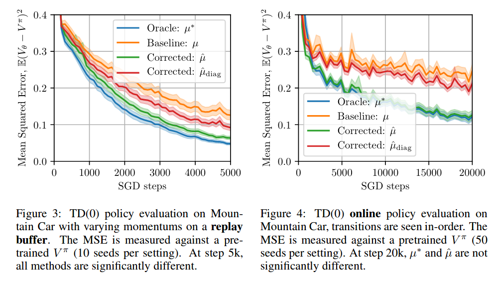
How well does this work in practice? For policy evaluation on small problems (Mountain Car, Cartpole, Acrobot) this works quite well. In our paper we find that the Taylor approximations are well aligned with the true gradients. We find that our method also corrects for value drift. This also seems to work on more complicated problems such as Atari, but the improvement is not as considerable.

Find more details in our paper!